注意
跳转到末尾 以下载完整的示例代码。
DGL 中的 Tree-LSTM
作者: Zihao Ye, Qipeng Guo, Minjie Wang, Jake Zhao, Zheng Zhang
警告
本教程旨在通过代码解释来深入了解论文。因此,此实现并未针对运行效率进行优化。有关推荐的实现,请参阅官方示例。
import os
在本教程中,您将学习如何使用 Tree-LSTM 网络进行情感分析。Tree-LSTM 是长短期记忆网络 (LSTM) 到树状网络拓扑的一种泛化。
Tree-LSTM 结构由 Kai 等人于 2015 年在 ACL 的一篇论文中首次提出:Improved Semantic Representations From Tree-Structured Long Short-Term Memory Networks。核心思想是通过将链式结构的 LSTM 扩展到树状结构的 LSTM,为语言任务引入句法信息。利用依存树和成分树技术来获得‘’潜在树‘’。
训练 Tree-LSTM 的挑战在于批处理——这是一种用于加速优化的机器学习标准技术。然而,由于树在本质上通常具有不同的形状,并行化并非易事。DGL 提供了一种替代方案。将所有树汇集到一个单一图中,然后根据每棵树的结构引导其上的消息传递。
任务和数据集
这里的步骤使用 dgl.data 中的 斯坦福情感树库 数据集。该数据集提供了细粒度的树级情感标注。共有五个类别:非常消极、消极、中立、积极和非常积极,它们表示当前子树中的情感。成分树中的非叶节点不包含单词,因此使用特殊的 PAD_WORD 标记来表示它们。在训练和推断期间,它们的嵌入将被掩码为全零。
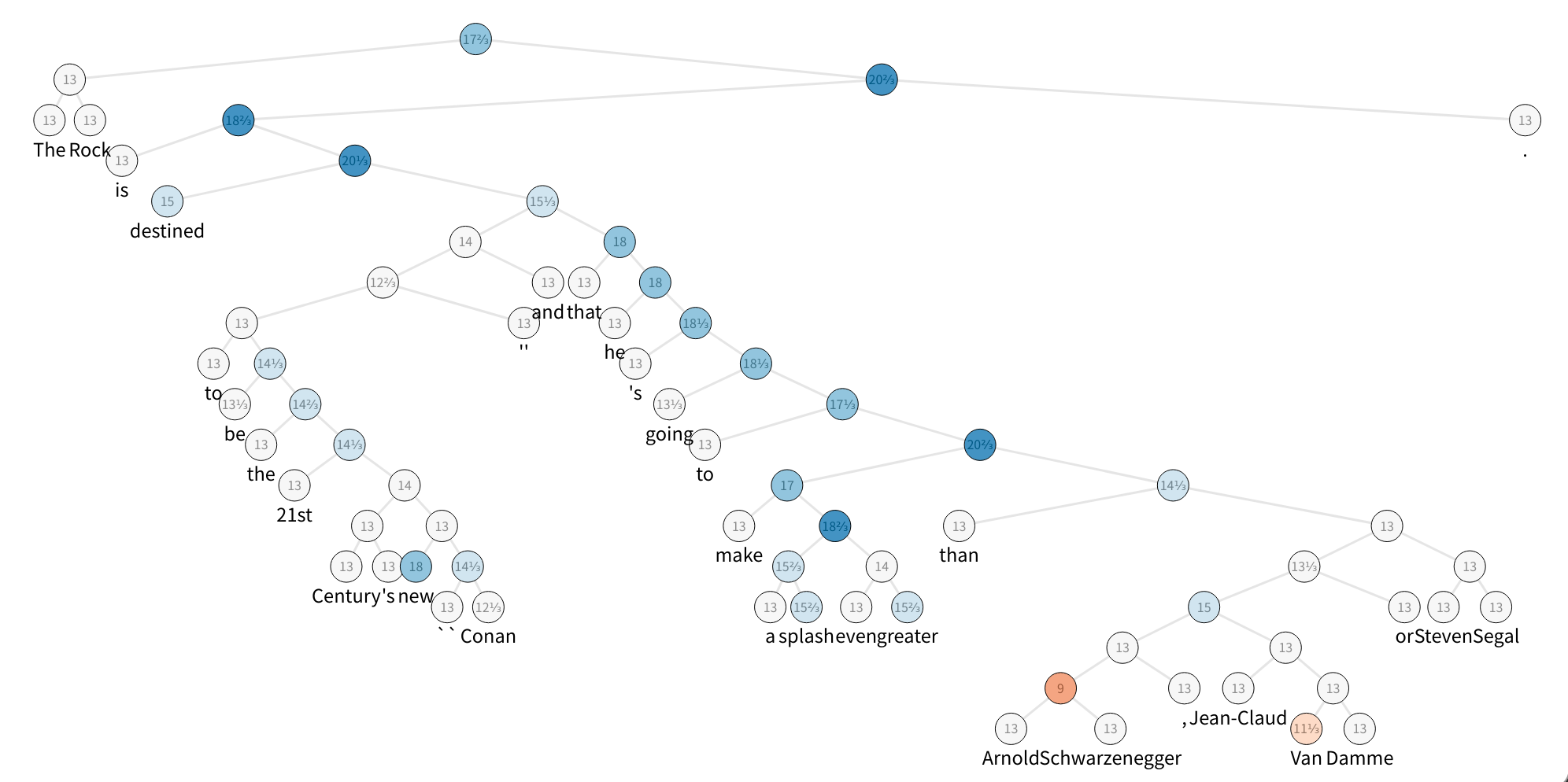
该图展示了 SST 数据集的一个示例,它是一棵成分解析树,其节点标记有情感。为了加快速度,构建了一个包含五个句子的微型数据集,并查看了第一个句子。
from collections import namedtuple

os.environ["DGLBACKEND"] = "pytorch"
import dgl
from dgl.data.tree import SSTDataset


SSTBatch = namedtuple("SSTBatch", ["graph", "mask", "wordid", "label"])

# Each sample in the dataset is a constituency tree. The leaf nodes
# represent words. The word is an int value stored in the "x" field.
# The non-leaf nodes have a special word PAD_WORD. The sentiment
# label is stored in the "y" feature field.
trainset = SSTDataset(mode="tiny")  # the "tiny" set has only five trees
tiny_sst = [tr for tr in trainset]
num_vocabs = trainset.vocab_size
num_classes = trainset.num_classes

vocab = trainset.vocab  # vocabulary dict: key -> id
inv_vocab = {
    v: k for k, v in vocab.items()
}  # inverted vocabulary dict: id -> word

a_tree = tiny_sst[0]
for token in a_tree.ndata["x"].tolist():
    if token != trainset.PAD_WORD:
        print(inv_vocab[token], end=" ")
import matplotlib.pyplot as plt
Downloading /root/.dgl/sst.zip from https://data.dgl.ai/dataset/sst.zip...

/root/.dgl/sst.zip:   0%|          | 0.00/930k [00:00<?, ?B/s]
/root/.dgl/sst.zip: 100%|██████████| 930k/930k [00:00<00:00, 29.6MB/s]
Extracting file to /root/.dgl/sst_c63ddc86
the rock is destined to be the 21st century 's new `` conan '' and that he 's going to make a splash even greater than arnold schwarzenegger , jean-claud van damme or steven segal .
步骤 1:批处理
使用 batch() API 将所有树添加到一张图中。
您可以阅读有关 batch() 定义的更多信息,或者跳到下一步:.. note
**Definition**: :func:`~dgl.batch` unions a list of :math:`B`
  :class:`~dgl.DGLGraph`\ s and returns a :class:`~dgl.DGLGraph` of batch
  size :math:`B`.

- The union includes all the nodes,
  edges, and their features. The order of nodes, edges, and features are
  preserved.

    - Given that you have :math:`V_i` nodes for graph
      :math:`\mathcal{G}_i`, the node ID :math:`j` in graph
      :math:`\mathcal{G}_i` correspond to node ID
      :math:`j + \sum_{k=1}^{i-1} V_k` in the batched graph.

    - Therefore, performing feature transformation and message passing on
      the batched graph is equivalent to doing those
      on all ``DGLGraph`` constituents in parallel.

- Duplicate references to the same graph are
  treated as deep copies; the nodes, edges, and features are duplicated,
  and mutation on one reference does not affect the other.
- The batched graph keeps track of the meta
  information of the constituents so it can be
  :func:`~dgl.batched_graph.unbatch`\ ed to list of ``DGLGraph``\ s.
步骤 2:使用消息传递 API 实现 Tree-LSTM 单元
研究人员提出了两种类型的 Tree-LSTM:Child-Sum Tree-LSTM 和 \(N\)-ary Tree-LSTM。在本教程中,您将重点关注将二叉 Tree-LSTM 应用于二值化成分树。此应用也称为成分 Tree-LSTM。使用 PyTorch 作为后端框架来设置网络。
在 N-ary Tree-LSTM 中,节点 \(j\) 处的每个单元维护一个隐藏表示 \(h_j\) 和一个记忆单元 \(c_j\)。单元 \(j\) 将输入向量 \(x_j\) 和子单元的隐藏表示:\(h_{jl}, 1\leq l\leq N\) 作为输入,然后通过以下方式更新其新的隐藏表示 \(h_j\) 和记忆单元 \(c_j\)
它可以分解为三个阶段:message_func、reduce_func 和 apply_node_func。
注意
apply_node_func 是之前未介绍过的新的节点 UDF。在 apply_node_func 中,用户指定如何处理节点特征,而不考虑边特征和消息。在 Tree-LSTM 的情况下,apply_node_func 是必需的,因为存在入度为 \(0\) 的(叶)节点,这些节点不会通过 reduce_func 进行更新。
import torch as th
import torch.nn as nn


class TreeLSTMCell(nn.Module):
    def __init__(self, x_size, h_size):
        super(TreeLSTMCell, self).__init__()
        self.W_iou = nn.Linear(x_size, 3 * h_size, bias=False)
        self.U_iou = nn.Linear(2 * h_size, 3 * h_size, bias=False)
        self.b_iou = nn.Parameter(th.zeros(1, 3 * h_size))
        self.U_f = nn.Linear(2 * h_size, 2 * h_size)

    def message_func(self, edges):
        return {"h": edges.src["h"], "c": edges.src["c"]}

    def reduce_func(self, nodes):
        # concatenate h_jl for equation (1), (2), (3), (4)
        h_cat = nodes.mailbox["h"].view(nodes.mailbox["h"].size(0), -1)
        # equation (2)
        f = th.sigmoid(self.U_f(h_cat)).view(*nodes.mailbox["h"].size())
        # second term of equation (5)
        c = th.sum(f * nodes.mailbox["c"], 1)
        return {"iou": self.U_iou(h_cat), "c": c}

    def apply_node_func(self, nodes):
        # equation (1), (3), (4)
        iou = nodes.data["iou"] + self.b_iou
        i, o, u = th.chunk(iou, 3, 1)
        i, o, u = th.sigmoid(i), th.sigmoid(o), th.tanh(u)
        # equation (5)
        c = i * u + nodes.data["c"]
        # equation (6)
        h = o * th.tanh(c)
        return {"h": h, "c": c}
步骤 3:定义遍历顺序
定义消息传递函数后,确定触发它们的正确顺序。这与 GCN 等模型显著不同,在 GCN 中,所有节点都同时从上游节点拉取消息。
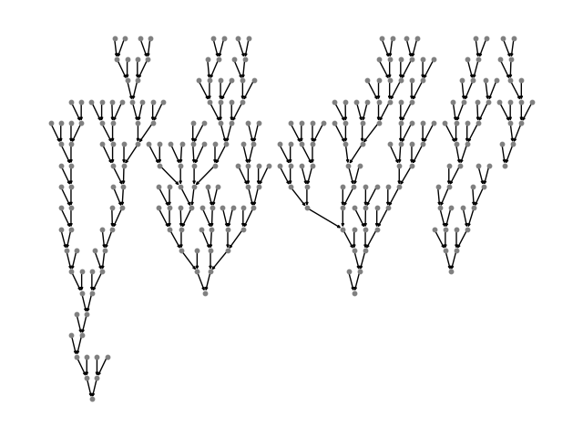
在 Tree-LSTM 的情况下,消息从树的叶节点开始,向上传播/处理直到到达根节点。可视化如下所示
DGL 定义了一个生成器来执行拓扑排序,每个项都是一个张量,记录了从底层到根节点的节点。通过检查以下内容的差异,可以了解并行化的程度
# to heterogenous graph
trv_a_tree = dgl.graph(a_tree.edges())
print("Traversing one tree:")
print(dgl.topological_nodes_generator(trv_a_tree))

# to heterogenous graph
trv_graph = dgl.graph(graph.edges())
print("Traversing many trees at the same time:")
print(dgl.topological_nodes_generator(trv_graph))
Traversing one tree:
(tensor([ 2,  3,  6,  8, 13, 15, 17, 19, 22, 23, 25, 27, 28, 29, 30, 32, 34, 36,
        38, 40, 43, 46, 47, 49, 50, 52, 58, 59, 60, 62, 64, 65, 66, 68, 69, 70]), tensor([ 1, 21, 26, 45, 48, 57, 63, 67]), tensor([24, 44, 56, 61]), tensor([20, 42, 55]), tensor([18, 54]), tensor([16, 53]), tensor([14, 51]), tensor([12, 41]), tensor([11, 39]), tensor([10, 37]), tensor([35]), tensor([33]), tensor([31]), tensor([9]), tensor([7]), tensor([5]), tensor([4]), tensor([0]))
Traversing many trees at the same time:
(tensor([  2,   3,   6,   8,  13,  15,  17,  19,  22,  23,  25,  27,  28,  29,
         30,  32,  34,  36,  38,  40,  43,  46,  47,  49,  50,  52,  58,  59,
         60,  62,  64,  65,  66,  68,  69,  70,  74,  76,  78,  79,  82,  83,
         85,  88,  90,  92,  93,  95,  96, 100, 102, 103, 105, 109, 110, 112,
        113, 117, 118, 119, 121, 125, 127, 129, 130, 132, 133, 135, 138, 140,
        141, 142, 143, 150, 152, 153, 155, 158, 159, 161, 162, 164, 168, 170,
        171, 174, 175, 178, 179, 182, 184, 185, 187, 189, 190, 191, 192, 195,
        197, 198, 200, 202, 205, 208, 210, 212, 213, 214, 216, 218, 219, 220,
        223, 225, 227, 229, 230, 232, 235, 237, 240, 242, 244, 246, 248, 249,
        251, 253, 255, 256, 257, 259, 262, 263, 267, 269, 270, 271, 272]), tensor([  1,  21,  26,  45,  48,  57,  63,  67,  77,  81,  91,  94, 101, 108,
        111, 116, 128, 131, 139, 151, 157, 160, 169, 173, 177, 183, 188, 196,
        211, 217, 228, 247, 254, 261, 268]), tensor([ 24,  44,  56,  61,  75,  89,  99, 107, 115, 126, 137, 149, 156, 167,
        181, 186, 194, 209, 215, 226, 245, 252, 266]), tensor([ 20,  42,  55,  73,  87, 124, 136, 154, 180, 207, 224, 243, 250, 265]), tensor([ 18,  54,  86, 123, 134, 148, 176, 206, 222, 241, 264]), tensor([ 16,  53,  84, 122, 172, 204, 239, 260]), tensor([ 14,  51,  80, 120, 166, 203, 238, 258]), tensor([ 12,  41,  72, 114, 165, 201, 236]), tensor([ 11,  39, 106, 163, 199, 234]), tensor([ 10,  37, 104, 147, 193, 233]), tensor([ 35,  98, 146, 231]), tensor([ 33,  97, 145, 221]), tensor([ 31,  71, 144]), tensor([9]), tensor([7]), tensor([5]), tensor([4]), tensor([0]))
调用 prop_nodes() 来触发消息传递
import dgl.function as fn
import torch as th

trv_graph.ndata["a"] = th.ones(graph.num_nodes(), 1)
traversal_order = dgl.topological_nodes_generator(trv_graph)
trv_graph.prop_nodes(
    traversal_order,
    message_func=fn.copy_u("a", "a"),
    reduce_func=fn.sum("a", "a"),
)

# the following is a syntax sugar that does the same
# dgl.prop_nodes_topo(graph)
注意
在调用 prop_nodes() 之前,请提前指定 message_func 和 reduce_func。在本例中,您可以看到内置的 copy-from-source 和 sum 函数作为消息函数,以及一个用于演示的 reduce 函数。
整合代码
以下是指定 Tree-LSTM 类的完整代码。
class TreeLSTM(nn.Module):
    def __init__(
        self,
        num_vocabs,
        x_size,
        h_size,
        num_classes,
        dropout,
        pretrained_emb=None,
    ):
        super(TreeLSTM, self).__init__()
        self.x_size = x_size
        self.embedding = nn.Embedding(num_vocabs, x_size)
        if pretrained_emb is not None:
            print("Using glove")
            self.embedding.weight.data.copy_(pretrained_emb)
            self.embedding.weight.requires_grad = True
        self.dropout = nn.Dropout(dropout)
        self.linear = nn.Linear(h_size, num_classes)
        self.cell = TreeLSTMCell(x_size, h_size)

    def forward(self, batch, h, c):
        """Compute tree-lstm prediction given a batch.

        Parameters
        ----------
        batch : dgl.data.SSTBatch
            The data batch.
        h : Tensor
            Initial hidden state.
        c : Tensor
            Initial cell state.

        Returns
        -------
        logits : Tensor
            The prediction of each node.
        """
        g = batch.graph
        # to heterogenous graph
        g = dgl.graph(g.edges())
        # feed embedding
        embeds = self.embedding(batch.wordid * batch.mask)
        g.ndata["iou"] = self.cell.W_iou(
            self.dropout(embeds)
        ) * batch.mask.float().unsqueeze(-1)
        g.ndata["h"] = h
        g.ndata["c"] = c
        # propagate
        dgl.prop_nodes_topo(
            g,
            message_func=self.cell.message_func,
            reduce_func=self.cell.reduce_func,
            apply_node_func=self.cell.apply_node_func,
        )
        # compute logits
        h = self.dropout(g.ndata.pop("h"))
        logits = self.linear(h)
        return logits


import torch.nn.functional as F
主循环
最后,您可以在 PyTorch 中编写训练范例。
from torch.utils.data import DataLoader

device = th.device("cpu")
# hyper parameters
x_size = 256
h_size = 256
dropout = 0.5
lr = 0.05
weight_decay = 1e-4
epochs = 10

# create the model
model = TreeLSTM(
    trainset.vocab_size, x_size, h_size, trainset.num_classes, dropout
)
print(model)

# create the optimizer
optimizer = th.optim.Adagrad(
    model.parameters(), lr=lr, weight_decay=weight_decay
)


def batcher(dev):
    def batcher_dev(batch):
        batch_trees = dgl.batch(batch)
        return SSTBatch(
            graph=batch_trees,
            mask=batch_trees.ndata["mask"].to(device),
            wordid=batch_trees.ndata["x"].to(device),
            label=batch_trees.ndata["y"].to(device),
        )

    return batcher_dev


train_loader = DataLoader(
    dataset=tiny_sst,
    batch_size=5,
    collate_fn=batcher(device),
    shuffle=False,
    num_workers=0,
)

# training loop
for epoch in range(epochs):
    for step, batch in enumerate(train_loader):
        g = batch.graph
        n = g.num_nodes()
        h = th.zeros((n, h_size))
        c = th.zeros((n, h_size))
        logits = model(batch, h, c)
        logp = F.log_softmax(logits, 1)
        loss = F.nll_loss(logp, batch.label, reduction="sum")
        optimizer.zero_grad()
        loss.backward()
        optimizer.step()
        pred = th.argmax(logits, 1)
        acc = float(th.sum(th.eq(batch.label, pred))) / len(batch.label)
        print(
            "Epoch {:05d} | Step {:05d} | Loss {:.4f} | Acc {:.4f} |".format(
                epoch, step, loss.item(), acc
            )
        )
TreeLSTM(
  (embedding): Embedding(19536, 256)
  (dropout): Dropout(p=0.5, inplace=False)
  (linear): Linear(in_features=256, out_features=5, bias=True)
  (cell): TreeLSTMCell(
    (W_iou): Linear(in_features=256, out_features=768, bias=False)
    (U_iou): Linear(in_features=512, out_features=768, bias=False)
    (U_f): Linear(in_features=512, out_features=512, bias=True)
  )
)
/dgl/python/dgl/core.py:82: DGLWarning: The input graph for the user-defined edge function does not contain valid edges
  dgl_warning(
Epoch 00000 | Step 00000 | Loss 440.4676 | Acc 0.2161 |
Epoch 00001 | Step 00000 | Loss 280.3035 | Acc 0.7253 |
Epoch 00002 | Step 00000 | Loss 1062.4580 | Acc 0.3150 |
Epoch 00003 | Step 00000 | Loss 226.0177 | Acc 0.6813 |
Epoch 00004 | Step 00000 | Loss 167.2298 | Acc 0.8425 |
Epoch 00005 | Step 00000 | Loss 164.9426 | Acc 0.8498 |
Epoch 00006 | Step 00000 | Loss 103.7912 | Acc 0.8864 |
Epoch 00007 | Step 00000 | Loss 136.7791 | Acc 0.8791 |
Epoch 00008 | Step 00000 | Loss 73.9224 | Acc 0.9304 |
Epoch 00009 | Step 00000 | Loss 61.6219 | Acc 0.9304 |
要在具有不同设置(例如 CPU 或 GPU)的完整数据集上训练模型,请参阅PyTorch 示例。还有一个 Child-Sum Tree-LSTM 的实现。
脚本总运行时间: (0 分钟 1.893 秒)