超图神经网络
本教程介绍什么是超图以及如何使用 DGL 的稀疏矩阵 API 构建超图神经网络。
![]()
[ ]:
# Install required packages.
import os
import torch
os.environ['TORCH'] = torch.__version__
os.environ['DGLBACKEND'] = "pytorch"

# Uncomment below to install required packages. If the CUDA version is not 11.8,
# check the https://dgl.ac.cn/pages/start.html to find the supported CUDA
# version and corresponding command to install DGL.
#!pip install dgl -f https://data.dgl.ai/wheels/cu118/repo.html > /dev/null
#!pip install torchmetrics > /dev/null

try:
    import dgl
    installed = True
except ImportError:
    installed = False
print("DGL installed!" if installed else "Failed to install DGL!")
超图
一个 超图 由节点和超边组成。与图中的边不同,一个超边可以连接任意数量的节点。例如,下图显示了一个包含 11 个节点和 5 条不同颜色绘制的超边的超图。 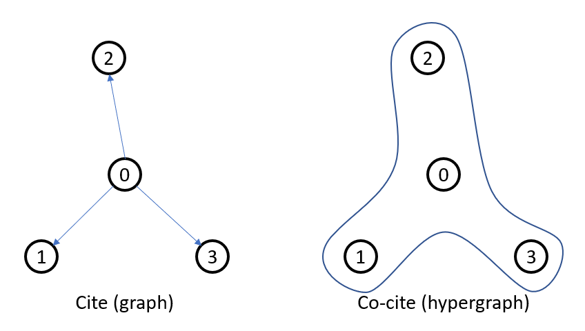
当数据集中的数据点之间的关系不是二元的时,超图特别有用。例如,在电子商务系统中,两个以上的产品可以一起被共同购买,因此共同购买的关系是 \(n\) 元的而不是二元的,因此最好将其描述为超图而不是普通图。
超图通常用其关联矩阵 \(H\) 来表征,其中行代表节点,列代表超边。如果超边 \(j\) 包含节点 \(i\),则条目 \(H_{ij}\) 为 1,否则为 0。例如,上图中的超图可以用一个 \(11 \times 5\) 的矩阵来表示,如下所示
可以通过指定两个张量 nodes 和 hyperedges 来构建超图关联矩阵,其中对于所有的 i,节点 ID nodes[i] 属于超边 ID hyperedges[i]。在上述情况下,关联矩阵可以按如下方式构建。
[ ]:
import dgl.sparse as dglsp
import torch

H = dglsp.spmatrix(
    torch.LongTensor([[0, 1, 2, 2, 2, 2, 3, 4, 5, 5, 5, 5, 6, 7, 7, 8, 8, 9, 9, 10],
                      [0, 0, 0, 1, 3, 4, 2, 1, 0, 2, 3, 4, 2, 1, 3, 1, 3, 2, 4, 4]])
)

print(H.to_dense())
tensor([[1., 0., 0., 0., 0.],
        [1., 0., 0., 0., 0.],
        [1., 1., 0., 1., 1.],
        [0., 0., 1., 0., 0.],
        [0., 1., 0., 0., 0.],
        [1., 0., 1., 1., 1.],
        [0., 0., 1., 0., 0.],
        [0., 1., 0., 1., 0.],
        [0., 1., 0., 1., 0.],
        [0., 0., 1., 0., 1.],
        [0., 0., 0., 0., 1.]])
超图中节点的度定义为包含该节点的超边数量。类似地,超图中超边的度定义为该超边包含的节点数量。在上述示例中,超边的度可以通过行向量的和计算(即全部为 4),而节点的度可以通过列向量的和计算。
[ ]:
node_degrees = H.sum(1)
print("Node degrees", node_degrees)

hyperedge_degrees = H.sum(0)
print("Hyperedge degrees", hyperedge_degrees)
Node degrees tensor([1., 1., 4., 1., 1., 4., 1., 2., 2., 2., 1.])
Hyperedge degrees tensor([4., 4., 4., 4., 4.])
超图神经网络 (HGNN) 层
HGNN 层的定义如下:
其中
\(H \in \mathbb{R}^{N \times M}\) 是具有 \(N\) 个节点和 \(M\) 条超边的超图的关联矩阵。
\(D_v \in \mathbb{R}^{N \times N}\) 是表示节点度的对角矩阵,其第 \(i\) 个对角线元素是 \(\sum_{j=1}^M H_{ij}\)。
\(D_e \in \mathbb{R}^{M \times M}\) 是表示超边度的对角矩阵,其第 \(j\) 个对角线元素是 \(\sum_{i=1}^N H_{ij}\)。
\(B \in \mathbb{R}^{M \times M}\) 是表示超边权重的对角矩阵,其第 \(j\) 个对角线元素是第 \(j\) 条超边的权重。在我们的示例中,\(B\) 是一个单位矩阵。
以下代码构建了一个两层的 HGNN。
[ ]:
import dgl.sparse as dglsp
import torch
import torch.nn as nn
import torch.nn.functional as F
import tqdm
from dgl.data import CoraGraphDataset
from torchmetrics.functional import accuracy


class HGNN(nn.Module):
    def __init__(self, H, in_size, out_size, hidden_dims=16):
        super().__init__()

        self.W1 = nn.Linear(in_size, hidden_dims)
        self.W2 = nn.Linear(hidden_dims, out_size)
        self.dropout = nn.Dropout(0.5)

        ###########################################################
        # (HIGHLIGHT) Compute the Laplacian with Sparse Matrix API
        ###########################################################
        # Compute node degree.
        d_V = H.sum(1)
        # Compute edge degree.
        d_E = H.sum(0)
        # Compute the inverse of the square root of the diagonal D_v.
        D_v_invsqrt = dglsp.diag(d_V**-0.5)
        # Compute the inverse of the diagonal D_e.
        D_e_inv = dglsp.diag(d_E**-1)
        # In our example, B is an identity matrix.
        n_edges = d_E.shape[0]
        B = dglsp.identity((n_edges, n_edges))
        # Compute Laplacian from the equation above.
        self.L = D_v_invsqrt @ H @ B @ D_e_inv @ H.T @ D_v_invsqrt

    def forward(self, X):
        X = self.L @ self.W1(self.dropout(X))
        X = F.relu(X)
        X = self.L @ self.W2(self.dropout(X))
        return X
加载数据
我们在示例中使用了 Cora 引文网络。但我们没有使用论文之间原始的“引用”关系,而是考虑论文之间的“共同引用”关系。我们从原始引文网络构建了一个超图,其中对于每一篇论文,我们构建了一条包含它引用的所有其他论文以及论文本身的超边。
请注意,以这种方式构建的超图的关联矩阵与原始图的邻接矩阵完全相同(加上一个用于自环的单位矩阵)。这是因为每条超边都与每篇论文一一对应。因此,我们可以直接使用图的邻接矩阵并加上一个单位矩阵,然后将其用作超图的关联矩阵。
[ ]:
def load_data():
    dataset = CoraGraphDataset()

    graph = dataset[0]
    indices = torch.stack(graph.edges())
    H = dglsp.spmatrix(indices)
    H = H + dglsp.identity(H.shape)

    X = graph.ndata["feat"]
    Y = graph.ndata["label"]
    train_mask = graph.ndata["train_mask"]
    val_mask = graph.ndata["val_mask"]
    test_mask = graph.ndata["test_mask"]
    return H, X, Y, dataset.num_classes, train_mask, val_mask, test_mask
训练和评估
现在我们可以编写训练和评估函数,如下所示。
[ ]:
def train(model, optimizer, X, Y, train_mask):
    model.train()
    Y_hat = model(X)
    loss = F.cross_entropy(Y_hat[train_mask], Y[train_mask])
    optimizer.zero_grad()
    loss.backward()
    optimizer.step()


def evaluate(model, X, Y, val_mask, test_mask, num_classes):
    model.eval()
    Y_hat = model(X)
    val_acc = accuracy(
        Y_hat[val_mask], Y[val_mask], task="multiclass", num_classes=num_classes
    )
    test_acc = accuracy(
        Y_hat[test_mask],
        Y[test_mask],
        task="multiclass",
        num_classes=num_classes,
    )
    return val_acc, test_acc


H, X, Y, num_classes, train_mask, val_mask, test_mask = load_data()
model = HGNN(H, X.shape[1], num_classes)
optimizer = torch.optim.Adam(model.parameters(), lr=0.001)

with tqdm.trange(500) as tq:
    for epoch in tq:
        train(model, optimizer, X, Y, train_mask)
        val_acc, test_acc = evaluate(
            model, X, Y, val_mask, test_mask, num_classes
        )
        tq.set_postfix(
            {
                "Val acc": f"{val_acc:.5f}",
                "Test acc": f"{test_acc:.5f}",
            },
            refresh=False,
        )

print(f"Test acc: {test_acc:.3f}")
Downloading /root/.dgl/cora_v2.zip from https://data.dgl.ai/dataset/cora_v2.zip...
Extracting file to /root/.dgl/cora_v2
Finished data loading and preprocessing.
  NumNodes: 2708
  NumEdges: 10556
  NumFeats: 1433
  NumClasses: 7
  NumTrainingSamples: 140
  NumValidationSamples: 500
  NumTestSamples: 1000
Done saving data into cached files.
100%|██████████| 500/500 [00:57<00:00, 8.70it/s, Val acc=0.77800, Test acc=0.78100]
Test acc: 0.781
关于完整的 HGNN 示例,请参考此处。